DATA-DRIVEN HOUSING INSIGHTS

Understanding House Prices Through Data.

Explore property characteristics, discover price patterns, and understand the results of two regression models developed using Python.

Explore Insights Model Results

Dataset Preview

A quick look at the housing dataset used in this project.

545
Housing records
13
Total columns
12
Predictor features
0
Recorded missing values

Project Overview

This project examines a residential housing dataset, explores how recorded property characteristics relate to price, and compares two linear regression models. The website presents the evidence and explains what the results can—and cannot—tell us.

Explore the dataset, study feature relationships, compare model performance, and review the main findings.

Key Finding

The multiple-feature model performed better than the area-only model on the recorded test split.

0.2729
Model A R² · Area only
0.6529
Model B R² · All 12 predictors
34.2%
Lower MAE for Model B

These are test-set results from one 80:20 split, not a guarantee of performance on other datasets or housing markets.

Dataset & Price Insights

The project uses Housing.csv. The target variable is price, and the remaining 12 columns are predictor features.

Dataset Overview

Dataset overview and verification
Item Verified result
Observations545
Columns13
Target variableprice
Predictor variables12
Missing values0 recorded null values across all 13 columns
Initial data types6 integer columns and 7 object/text columns
Recorded price range1,750,000 to 13,300,000 dataset units

Data source note: The supplied CSV and notebook do not document the dataset's geography, collection date, publisher, or price currency. Values are therefore presented in dataset units, without assigning a currency symbol.
Housing Feature Classification

Housing features and their role in the project
Group Columns Role in the analysis
Numerical area, bedrooms, bathrooms, stories, parking Descriptive statistics, grouped comparisons, and regression inputs.
Binary mainroad, guestroom, basement, hotwaterheating, airconditioning, prefarea Yes/No fields mapped to 1/0 for correlation and regression.
Categorical furnishingstatus Compared by category and encoded with One-Hot Encoding in Model B.
Target price House-price value described and predicted by the models.

Price Summary Statistics

These descriptive statistics summarise the distribution of the target variable, price.

Summary statistics for price (dataset units)
Statistic Value
Count545
Mean4,766,729
Median (50th percentile)4,340,000
Standard deviation1,870,440
25th percentile3,430,000
75th percentile5,740,000
Minimum1,750,000
Maximum13,300,000

The mean is higher than the median. The middle half of recorded prices lies between 3,430,000 and 5,740,000 dataset units.

Price Distribution and Potential Outliers

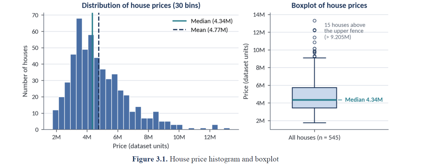
Histogram and boxplot showing a right-skewed distribution of house prices and potential high-price outliers.
Figure 3.1. House-price histogram and boxplot.

The histogram shows a concentration of observations in the lower-to-middle price range and a longer tail towards higher values. The boxplot identifies 15 of 545 houses (approximately 2.8%) above the upper fence of 9,205,000 dataset units. These are potential outliers under the boxplot rule, not confirmed data errors. The project retained them rather than removing them without further investigation.

Price and Area Relationship

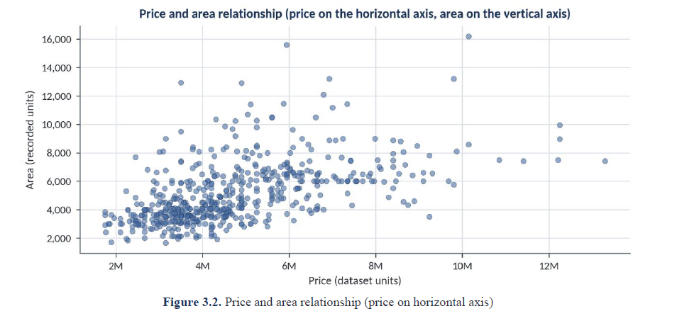
Scatter plot showing the relationship between house price and area. In the original notebook, price is on the horizontal axis and area is on the vertical axis.
Figure 3.2. Price and area relationship. The original notebook places price on the horizontal axis and area on the vertical axis.

The point cloud indicates a positive association: larger recorded areas are often observed alongside higher prices. The spread around this general pattern shows that area alone does not account for every price difference.

Furnishing-Status Analysis

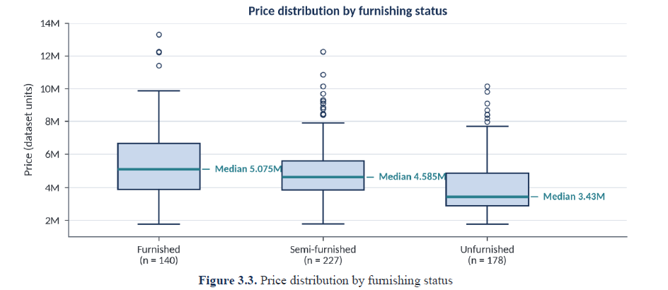
Boxplot comparing house-price distributions for furnished, semi-furnished, and unfurnished properties.
Figure 3.3. Price distribution by furnishing status.
Furnishing groups and approximate median prices
Furnishing status Number of houses Median price (approx.)
Furnished1405,075,000
Semi-furnished2274,585,000
Unfurnished1783,430,000

Furnished properties have the highest recorded median, followed by semi-furnished and unfurnished properties. The distributions overlap and vary within each group. This is an association in the dataset; it does not establish that furnishing causes a higher price or isolate its effect from other characteristics.

Feature Analysis

Explore how recorded housing characteristics relate to property prices.

Correlation Analysis

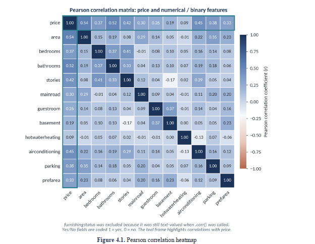
Pearson's correlation coefficient (r) describes the direction and strength of a linear association between two numerical variables. It ranges from −1 to +1. Values near +1 indicate a positive linear association, values near −1 indicate a negative linear association, and values near zero indicate a weak linear association. Correlation is not evidence of causation and does not, by itself, measure overall predictive importance.

The six Yes/No fields were mapped to 1/0 before the correlation calculation. The furnishingstatus column was excluded from the matrix because it was still text-valued when the correlation matrix was calculated. The heatmap coefficients are rounded to two decimal places.

Pearson correlation coefficients with price
Rank Feature Pearson r
1Area0.54
2Bathrooms0.52
3Air conditioning0.45
4Stories0.42
5Parking0.38
6Bedrooms0.37
7Preferred area0.33
8Mainroad0.30
9Guestroom0.26
10Basement0.19
11Hot water heating0.09
Annotated Pearson correlation heatmap showing correlations among the numerical and binary housing features, including price.
Figure 4.1. Pearson correlation heatmap. Furnishing status is not part of the matrix.

Area and bathrooms have the strongest positive pairwise correlations with price. Air conditioning and stories follow; hot water heating has the weakest positive correlation (0.09). These are pairwise linear relationships. They do not account for interactions among features and do not establish that a feature causes a price change.

Numerical Feature Analysis

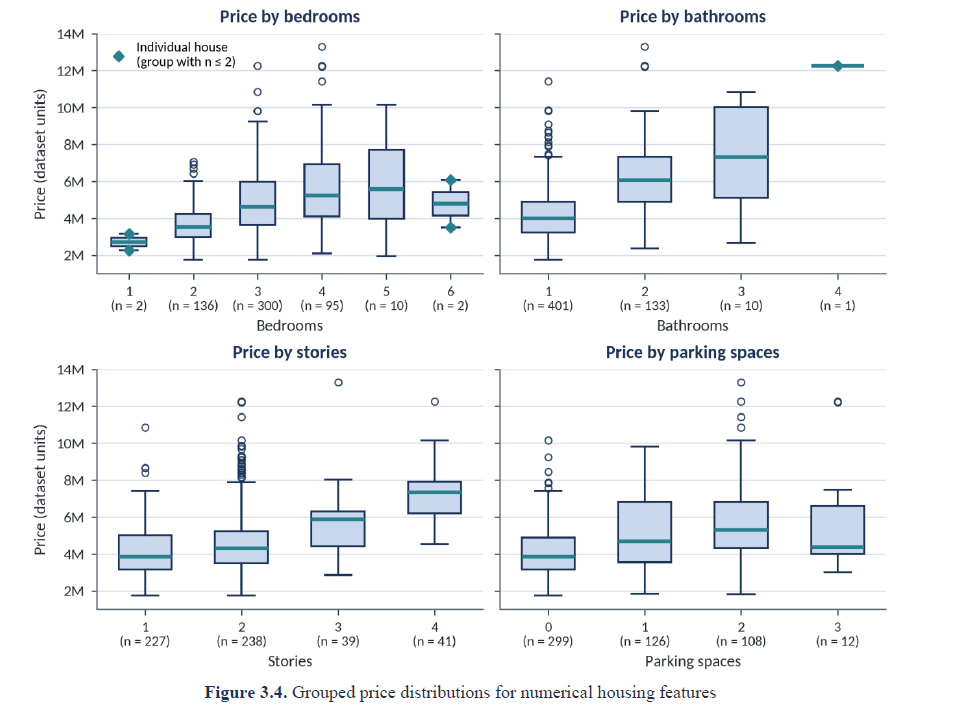
The project inspected the values and frequencies of numerical housing attributes and compared price distributions across their groups.

Frequencies of numerical housing attributes
Feature 0 1 2 3 4 5 6
Bedrooms—213630095102
Bathrooms—401133101——
Stories—2272383941——
Parking spaces29912610812———
Grouped boxplots comparing house-price distributions across bedroom, bathroom, story, and parking categories.
Figure 3.4. Grouped price distributions for numerical housing features.
  • Three-bedroom houses are the most common group: 300 of 545 records.
  • The one-bedroom and six-bedroom groups each contain only two houses.
  • The four-bathroom category contains one record, so its plotted value does not represent a stable group distribution.
  • Median price generally rises across one to four stories: approximately 3.85, 4.31, 5.87, and 7.35 million dataset units.
  • The two-parking-space group has the highest recorded median; the zero-parking group has the lowest. The three-space category contains 12 records.

Binary Feature Analysis

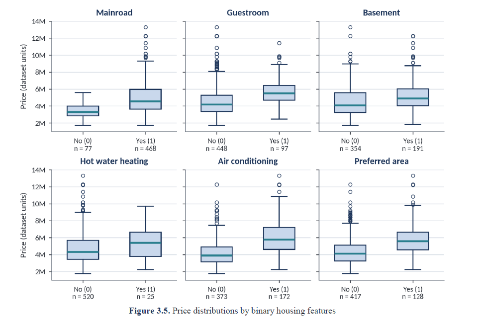
The project compared price distributions for the zero (No) and one (Yes) groups of each binary feature. Group sizes are uneven.

Frequencies of binary housing attributes
Feature Value 0 (No) Value 1 (Yes)
Mainroad77468
Guestroom44897
Basement354191
Hot water heating52025
Air conditioning373172
Preferred area417128
Grouped boxplots comparing price distributions for Yes and No groups across six binary housing features.
Figure 3.5. Price distributions by binary housing features.

The Yes group has a higher median in the recorded boxplots for mainroad, guestroom, basement, air conditioning, preferred-area status, and hot water heating. Only 25 houses have hot water heating. The price distributions overlap, so these are descriptive associations rather than causal effects.

Model Evaluation

Compare the two regression models and understand how well they estimated prices for the held-out test observations.

Evaluation Setup

Both models were evaluated using an 80:20 train-test split with random_state=42. This produced 436 training observations and 109 test observations. The same split configuration was used for both models.

  • Model A: Simple Linear Regression using area as its only predictor.
  • Model B: Multiple Linear Regression using all 12 predictor columns, including area.

How Model B Handles Furnishing Status

Furnishing status contains three categories: furnished, semi-furnished, and unfurnished. The project used One-Hot Encoding rather than assigning arbitrary numeric ranks to these categories. A ColumnTransformer applied the encoding to furnishingstatus, while the other predictor columns passed through. A Scikit-learn Pipeline connected this preprocessing step to the linear regression model.

The encoder was fitted as part of the pipeline using the training data, then applied to the test data using the learned category representation.

Model Performance Comparison

Model A and Model B performance on the same 109-house test subset
Metric Model A: Area only Model B: All 12 predictors Change (B relative to A)
MAE1,474,748.1338970,043.4039−34.2%
RMSE1,917,103.70211,324,506.9601−30.9%
R²0.27290.6529+0.380

Model B reduces MAE by approximately 34.2% and RMSE by approximately 30.9%. R² increases from 0.2729 to 0.6529, a gain of about 0.380. This is an empirical result for the recorded test split; it does not establish that every added feature is independently useful or causes a price change.

Sample Test Predictions

The following five rows illustrate individual predictions from the test set. They are examples, not a substitute for metrics calculated across all 109 test observations.

First five recorded test predictions (dataset units)
Row index Actual price Model A prediction Model B prediction
3164,060,0005,024,0605,164,654
776,650,0005,279,4987,224,722
3603,710,0004,232,2033,109,863
906,440,0004,640,9034,612,075
4932,800,0004,198,1443,294,646

The examples include both overestimates and underestimates for each model.

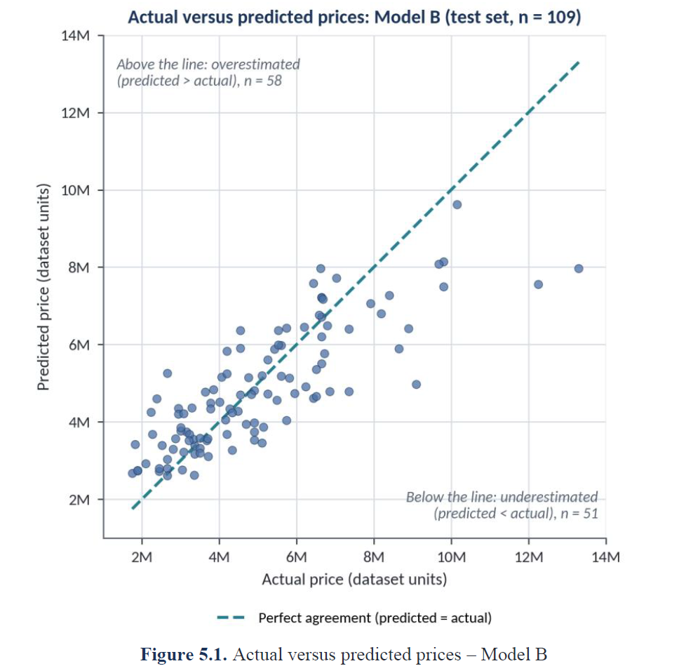
Actual vs Predicted Prices — Model B

Scatter plot comparing actual test prices on the horizontal axis with Model B predicted prices on the vertical axis, including a diagonal perfect-agreement line.
Figure 5.1. Actual versus predicted prices for Model B.

The horizontal axis shows actual test prices and the vertical axis shows Model B predictions. The dashed diagonal represents perfect agreement. Points above the line are overestimates; points below it are underestimates. Of the 109 test houses, 58 lie above the line and 51 lie below it. Some expensive houses are substantially underestimated.

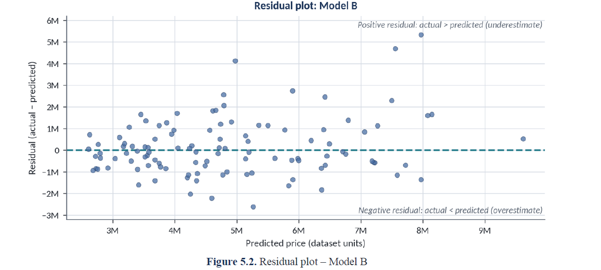
Residual Analysis — Model B

A residual is calculated as actual price minus predicted price: residual = actual − predicted. A positive residual indicates underestimation; a negative residual indicates overestimation; a residual near zero indicates a closer prediction.

Residual plot for Model B showing residuals against predicted prices with a horizontal zero-residual reference line.
Figure 5.2. Residual plot for Model B.

The plot contains residuals on both sides of zero, including comparatively large positive and negative values. The spread appears to widen at some higher predicted-price levels, suggesting that prediction variability may be larger for more expensive properties. This visual pattern could be consistent with heteroscedasticity, but no formal statistical test was recorded, so it is not treated as a confirmed assumption violation.

Explore Findings

Review the main findings from the housing data analysis and regression experiments.

Key Insights

0.54
Area correlation
Highest positive pairwise correlation with price among the features in the correlation table.
0.52
Bathrooms correlation
Second-highest positive pairwise correlation with price.
0.6529
Model B R²
Test-set coefficient of determination.
34.2%
MAE reduction
Reduction compared with Model A on the same test split.

What Do the Findings Tell Us?

  1. Dataset: The dataset contains 545 observations and 13 columns, with no recorded null values.
  2. Price distribution: Prices are right-skewed, with potential high-price outliers retained in the analysis.
  3. Feature relationships: Area (0.54) and bathrooms (0.52) have the strongest positive pairwise correlations with price among the analysed numerical and binary features.
  4. Group comparisons: Furnishing, layout, amenities, and access groups show differences in median prices, but distributions overlap and group sizes are uneven.
  5. Model comparison: Model B produces lower MAE and RMSE and a higher R² than Model A on the same test split.
  6. Remaining error: Actual-versus-predicted and residual plots show that individual predictions can still be materially inaccurate.

Insights for Buyers and Sellers

For buyers: Consider several property characteristics when comparing houses. A single characteristic or model estimate does not provide a complete assessment of a property.

For sellers: Recorded property characteristics can help describe differences in prices within this dataset. The analysis does not establish the exact market value of an individual property.

These are practical interpretations of the project findings, not tested buyer or seller recommendation services.

Interactive Exploration

Explore housing feature relationships, compare regression models, and understand prediction errors through interactive tools.

1. Feature Explorer

Select a housing feature to explore its correlation with house price.

Selected feature: Area

Correlation: 0.54

Relationship: Positive

Area has the strongest positive pairwise correlation with price among the listed features.

2. Model Comparison

Select an evaluation metric to compare both models.

Model A: 1,474,748.1338

Model B: 970,043.4039

Mean Absolute Error measures average absolute prediction error.

Model B has a lower MAE on the recorded test split.

3. Residual Calculator

Enter an actual price and a predicted price to understand the prediction error.

Residual: Not calculated

Enter both prices to understand the result.

Note: This calculator explains residuals using user-entered values. It does not generate predictions using the trained Python model.

These interactive tools explore existing project results. They do not provide live house-price predictions.

Limitations

Understanding the boundaries of the dataset and the regression results is essential before interpreting the findings.

Dataset Limitations

  • The dataset contains 545 observations and a limited set of 12 predictor features.
  • House age and construction year are not included.
  • The dataset's provenance, geography, collection date, and price currency are not documented in the supplied CSV or notebook.
  • Category frequencies are unequal. The one-bedroom and six-bedroom groups each contain two houses, the four-bathroom category contains one house, and only 25 houses have hot water heating.

Model Limitations

  • Model B achieved an R² of 0.6529 on the recorded test set; unexplained variation remains. R² should not be interpreted as a percentage of prediction accuracy.
  • Model B's MAE is approximately 970,043 in the dataset's price units.
  • Evaluation used one 80:20 train-test split with random_state=42.
  • No cross-validation, hyperparameter tuning, or external validation was recorded.
  • Some expensive houses remain difficult to predict.
  • The residual plot suggests a possible wider spread at higher predicted prices, but no formal heteroscedasticity test was recorded.
  • A detailed investigation of the categories associated with the largest prediction errors was not completed.

Responsible Use of Predictions

  • Predicted prices are estimates, not guaranteed market values.
  • The model is not a professional property valuation tool.
  • Predictions should not be the only information used for property-related decisions.
  • The dataset does not include every factor that can influence house prices.

Conclusion and Future Scope

Project Conclusion

The project applied Python to the inspection, preparation, exploratory analysis, correlation analysis, and predictive modelling of a residential housing dataset. Pandas operations established the dataset structure and confirmed the absence of recorded missing values. Matplotlib and Seaborn visualisations described the target distribution and compared prices across property characteristics. Mapping of binary fields and One-Hot Encoding of furnishing status prepared the features for correlation and regression.

The Simple Linear Regression model using area alone achieved an MAE of 1,474,748.1338, an RMSE of 1,917,103.7021, and an R² of 0.2729. The Multiple Linear Regression model using all 12 predictor features achieved an MAE of 970,043.4039, an RMSE of 1,324,506.9601, and an R² of 0.6529 on the same test configuration. The multiple-feature model therefore performed better in the recorded experiment. Because substantial errors remain and evaluation used a single split, the model should be treated as a data-driven estimation exercise rather than a guaranteed property valuation system.

Future Scope

The thesis identifies the following possible extensions. These were proposed future activities and were not implemented in the submitted Python notebook:

  • Strengthen validation through k-fold cross-validation and repeated train-test splits.
  • Compare additional regression algorithms.
  • Tune model parameters using a defined validation procedure.
  • Investigate large residuals and sparse feature categories more systematically.
  • Test supported feature-engineering approaches if additional source data becomes available.
  • Save and load the fitted pipeline with Joblib for a later controlled application.
  • Explore a separate future integration of the trained model with a Flask and HTML/CSS/JavaScript interface.

The current website is a separate presentation of completed findings. Its planned JavaScript interactions will explore existing results; they will not connect to the trained Python model or provide live predictions.